Deploying Manufacturing Analytics for Yield Optimization
Deploying Manufacturing Analytics for Yield Optimization: A Financial and Operational Plan Manufacturing analytics uses operational data to reduce direct material usage variances while improving labor efficiency and machine utilization. From a financial controllership perspective, improving yield is the most direct method for increasing gross margins without altering pricing structures. It also aligns actual production with…
Deploying Manufacturing Analytics for Yield Optimization: A Financial and Operational Plan
Manufacturing analytics uses operational data to reduce direct material usage variances while improving labor efficiency and machine utilization. From a financial controllership perspective, improving yield is the most direct method for increasing gross margins without altering pricing structures. It also aligns actual production with standard bill of materials (BOM) rollups, reducing unallocated overhead and making absorption costing metrics easier to reconcile.
Financial & Operational Prerequisites: What You Need
An auditable, ROI-positive deployment requires connected operational technology (OT) and information technology (IT) control environments.
- Hardware and Industrial IoT (IIoT) Sensors: Deployment requires PLCs and sensors (temperature, pressure, vibration). Accounting treatment: Hardware and installation costs are typically capitalized (CAPEX) and depreciated over the machinery’s useful life, affecting EBITDA but preserving short-term cash flow if financed appropriately.
- Production-Grade Data Infrastructure: A secure architecture utilizing edge computing for latency-sensitive controls or cloud storage. Accounting treatment: Cloud-based infrastructure is treated as an operating expense (OPEX). Review software-as-a-service (SaaS) agreements for predictable monthly burn rates.
- Cross-Functional Implementation Team: Plant managers and process engineers, supported by IT architects. Implementation Tip: Track internal IT/Engineering hours dedicated to system development. Under ASC 350-40 (Internal-Use Software), applicable payroll costs may be capitalized during the application development stage, reducing current-period P&L expense.
- Clearly Defined Yield Baseline: Before deployment, finance must lock the current standard costing baseline. Document historical production yield and allowable scrap percentages within existing BOMs, along with actual historical unfavorable usage variances.
Step 1: Data Collection and System Integration
- Auditing Existing Data Sources: Conduct a gap analysis between the ERP (e.g., SAP, Dynamics) and SCADA systems. Typically, financial controllers discover that shop floor subledgers do not reconcile with the general ledger without manual month-end journal entries.
- Connecting IT and OT Systems: Establish a unified pipeline. Production data must flow from the factory floor directly into the ERP’s perpetual inventory module. That connection supports internal controls over inventory valuation and helps eliminate phantom inventory during physical stocktakes.
- Data Cleansing and Standardization: Raw PLC data is noisy. Implement strict protocols to filter anomalies. If unverified sensor spikes trigger automated scrap write-offs, it will create material misstatements in standard cost variances, complicating the audit trail.
Step 2: Applying Predictive Modeling for Yield Optimization
- Analytical Model Selection: Deploy machine learning models that target high-cost variance drivers. For example, regression models that predict output rates directly influence labor efficiency variances and fixed overhead absorption rates.
- Model Training for Yield Detractors: Feed the algorithm with historical data. Use the model to correlate environmental/machine conditions (e.g., ambient humidity, RPMs) with increased scrap rates.
- Predictive Outcome Testing and Validation: Test models in a sandbox environment parallel to live production. Finance must maintain a pro forma P&L alongside the sandbox to quantify the financial impact of the model’s prescribed actions before pushing it to the live OT environment.
Target State: Maintaining Higher Yields
- Real-Time Production Dashboards: Replace retroactive variance reporting with real-time visibility. Display overall equipment effectiveness (OEE) and live yield metrics to operators. Finance can then replace a 15-day month-end variance review with a 5-day close, removing most manual WIP recalculations.
- Automating Corrective Actions: With prescriptive analytics, the system can adjust machine setpoints autonomously. Use these adjustments to prevent unfavorable material usage variances before the raw materials are consumed.
- Continuous Improvement Loop: Once yield stabilizes, finance should revise standard costs. Tightening the scrap allowances in the BOM rollup lowers the standard cost of goods sold (COGS), giving the commercial team more pricing flexibility.
Process Manufacturing Scenario: Aluminum Casting Plant
Background: A $40M turnover aluminum die-casting facility operating on a standard costing system.
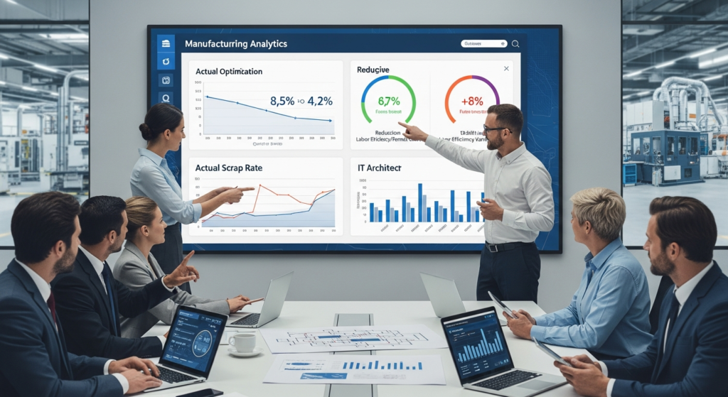
The Problem: The standard BOM allows for a 5% scrap rate (porosity and short shots). Actual scrap was running at 8.5%. The 3.5% unfavorable material usage variance was reducing gross margin by approximately $35,000 per month due to wasted aluminum ingots and energy (remelting costs).
The Intervention: Deployed thermal IIoT sensors on the die-cast molds and integrated them with a cloud-based analytics engine to predict thermal degradation before metal injection.
Financial Impact Matrix:
| Metric | Pre-Deployment (Baseline) | Post-Deployment (Month 6) | Financial Impact |
|---|---|---|---|
| Actual Scrap Rate | 8.5% | 4.2% | Favorable variance to BOM |
| Furnace Energy/Remelt | $18,000/mo | $8,500/mo | $9,500/mo OPEX reduction |
| Labor Efficiency Variance | -$12,000/mo | +$2,000/mo | $14,000/mo improvement |
| Unfavorable Mat. Variance | -$35,000/mo | $0 (Beat Standard) | $35,000/mo savings |
| Annualized P&L Impact | N/A | N/A | +$702,000 EBIT improvement |
Implementation Note: Total project CAPEX + OPEX was $185,000. The project paid back in just under 3.2 months.
Common Mistakes to Avoid
- Operating in Data Silos (The “Reconciliation Problem”): Keeping quality control databases segregated from ERP inventory modules. If a machine rejects 50 units but the ERP isn’t updated in real-time, the perpetual inventory remains overstated. This necessitates massive, unexpected write-downs during cycle counting or annual stocktakes.
- Overlooking Shop Floor User Adoption: Bypassing operator workflows ruins data integrity. If operators find the analytics interface cumbersome, they will manually override PLC locks. System reliability depends on the shop floor’s willingness to input accurate data.
- Scaling Too Quickly Without a Proof of Concept: Attempting a plant-wide deployment results in severe CAPEX blowouts. Implementation Tip: Apply the Pareto principle. Identify the top 20% of SKUs that generate 80% of your gross margin. Deploy analytics exclusively on the lines producing those SKUs to fund subsequent rollouts with realized cash flow.
Frequently Asked Questions
- What is the typical ROI timeline for a manufacturing analytics deployment?
In plants with $10M–$60M turnover, initial ROI typically lands within 4 to 8 months. Payback is usually driven by reductions in direct material scrap and labor inefficiency variances resulting from minimized unplanned downtime. - How does manufacturing analytics differ from traditional Business Intelligence (BI)?
Traditional BI is strictly descriptive; it tells the CFO what the variance was at month-end. Manufacturing analytics predicts likely losses and prescribes adjustments before those losses reach the ledger.